These are the currently implemented distributions.
| Name | univariateML function | Package | Parameters | Support |
|---|---|---|---|---|
| Cauchy distribution | mlcauchy |
stats |
location,scale
|
\(\mathbb{R}\) |
| Gumbel distribution | mlgumbel |
extraDistr |
mu, sigma
|
\(\mathbb{R}\) |
| Laplace distribution | mllaplace |
extraDistr |
mu, sigma
|
\(\mathbb{R}\) |
| Logistic distribution | mllogis |
stats |
location,scale
|
\(\mathbb{R}\) |
| Normal distribution | mlnorm |
stats |
mean, sd
|
\(\mathbb{R}\) |
| Beta prime distribution | mlbetapr |
extraDistr |
shape1, shape2
|
\((0, \infty)\) |
| Exponential distribution | mlexp |
stats | rate |
\([0, \infty)\) |
| Gamma distribution | mlgamma |
stats |
shape,rate
|
\((0, \infty)\) |
| Inverse gamma distribution | mlinvgamma |
extraDistr |
alpha, beta
|
\((0, \infty)\) |
| Inverse Gaussian distribution | mlinvgauss |
actuar |
mean, shape
|
\((0, \infty)\) |
| Inverse Weibull distribution | mlinvweibull |
actuar |
shape, rate
|
\((0, \infty)\) |
| Log-logistic distribution | mlllogis |
actuar |
shape, rate
|
\((0, \infty)\) |
| Log-normal distribution | mllnorm |
stats |
meanlog, sdlog
|
\((0, \infty)\) |
| Lomax distribution | mllomax |
extraDistr |
lambda, kappa
|
\([0, \infty)\) |
| Rayleigh distribution | mlrayleigh |
extraDistr | sigma |
\([0, \infty)\) |
| Weibull distribution | mlweibull |
stats |
shape,scale
|
\((0, \infty)\) |
| Log-gamma distribution | mllgamma |
actuar |
shapelog, ratelog
|
\((1, \infty)\) |
| Pareto distribution | mlpareto |
extraDistr |
a, b
|
\([b, \infty)\) |
| Beta distribution | mlbeta |
stats |
shape1,shape2
|
\((0, 1)\) |
| Kumaraswamy distribution | mlkumar |
extraDistr |
a, b
|
\((0, 1)\) |
| Logit-normal | mllogitnorm |
logitnorm |
mu, sigma
|
\((0, 1)\) |
| Uniform distribution | mlunif |
stats |
min, max
|
\([\min, \max]\) |
| Power distribution | mlpower |
extraDistr |
alpha, beta
|
\([0, a)\) |
This package follows a naming convention for the ml*** functions. To access the documentation of the distribution associated with an ml*** function, write package::d***. For instance, to find the documentation for the log-gamma distribution write
Problematic Distributions
Lomax Distribution
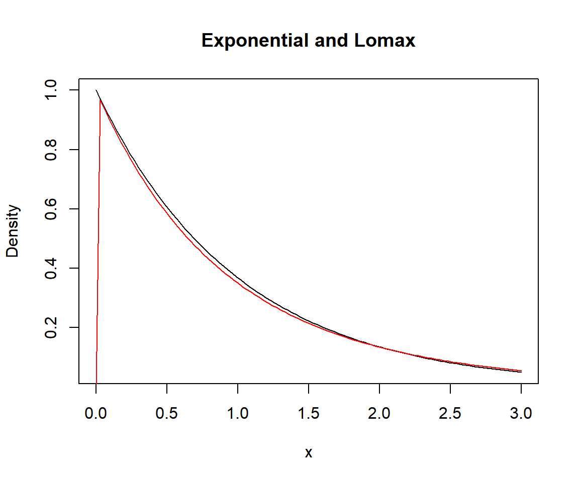
The maximum likelihood estimator of the Lomax distribution frequently fails to exist. For assume \(\kappa\to\lambda^{-1}\overline{x}^{-1}\) and \(\lambda\to0\). The density \(\lambda\kappa\left(1+\lambda x\right)^{-\left(\kappa+1\right)}\) is approximately equal to \(\lambda\kappa\left(1+\lambda x\right)^{-\left(\lambda^{-1}\overline{x}^{-1}+1\right)}\) when \(\lambda\) is small enough. Since \(\lambda\kappa\left(1+\lambda x\right)^{-\left(\lambda^{-1}\overline{x}^{-1}+1\right)}\to\overline{x}^{-1}e^{-\overline{x}^{-1}x}\), the density converges to an exponential density.
eps = 0.1
x = seq(0, 3, length.out = 100)
plot(dexp, 0, 3, xlab = "x", ylab = "Density", main = "Exponential and Lomax")
lines(x, extraDistr::dlomax(x, lambda = eps, kappa = 1/eps), col = "red")