## Loading required package: copula## Loading required package: dplyr##
## Attaching package: 'dplyr'## The following objects are masked from 'package:stats':
##
## filter, lag## The following objects are masked from 'package:base':
##
## intersect, setdiff, setequal, unionThis vignette shows how to model multivariate distributions with copulas using univariateML and the copula package.
A copula is a function describing the dependency among a set of one-dimensional distributions. If both the marginal distributions and the copula is known, the entire multivariate distribution is known too.
Suppose we look at a multivariate distribution as the pair of a copula and its marginals. Then a natural model selection using is to
1.) select the marginal distributions using the AIC; 2.) select a copula using the marginal data transformed to the unit interval, again using the AIC.
This two-step procedure is commonly used due to its simplicity. The procedure must be carried out this order since the marginal data cannot be transformed to the unit interval unless we know the marginal distributions.
The univariateML can be used for task 1, while the copula package can be used to do task 2.
Abalone data
The abalone data set is included in this package. It consists of \(9\) physical measurements of \(4177\) sea snails.
## # A tibble: 6 x 9
##   sex   length diameter height whole_weight shucked_weight viscera_weight
##   <fct>  <dbl>    <dbl>  <dbl>        <dbl>          <dbl>          <dbl>
## 1 M      0.455    0.365  0.095        0.514         0.224          0.101
## 2 M      0.35     0.265  0.09         0.226         0.0995         0.0485
## 3 F      0.53     0.42   0.135        0.677         0.256          0.142
## 4 M      0.44     0.365  0.125        0.516         0.216          0.114
## 5 I      0.33     0.255  0.08         0.205         0.0895         0.0395
## 6 I      0.425    0.3    0.095        0.352         0.141          0.0775
## # ... with 2 more variables: shell_weight <dbl>, rings <int>
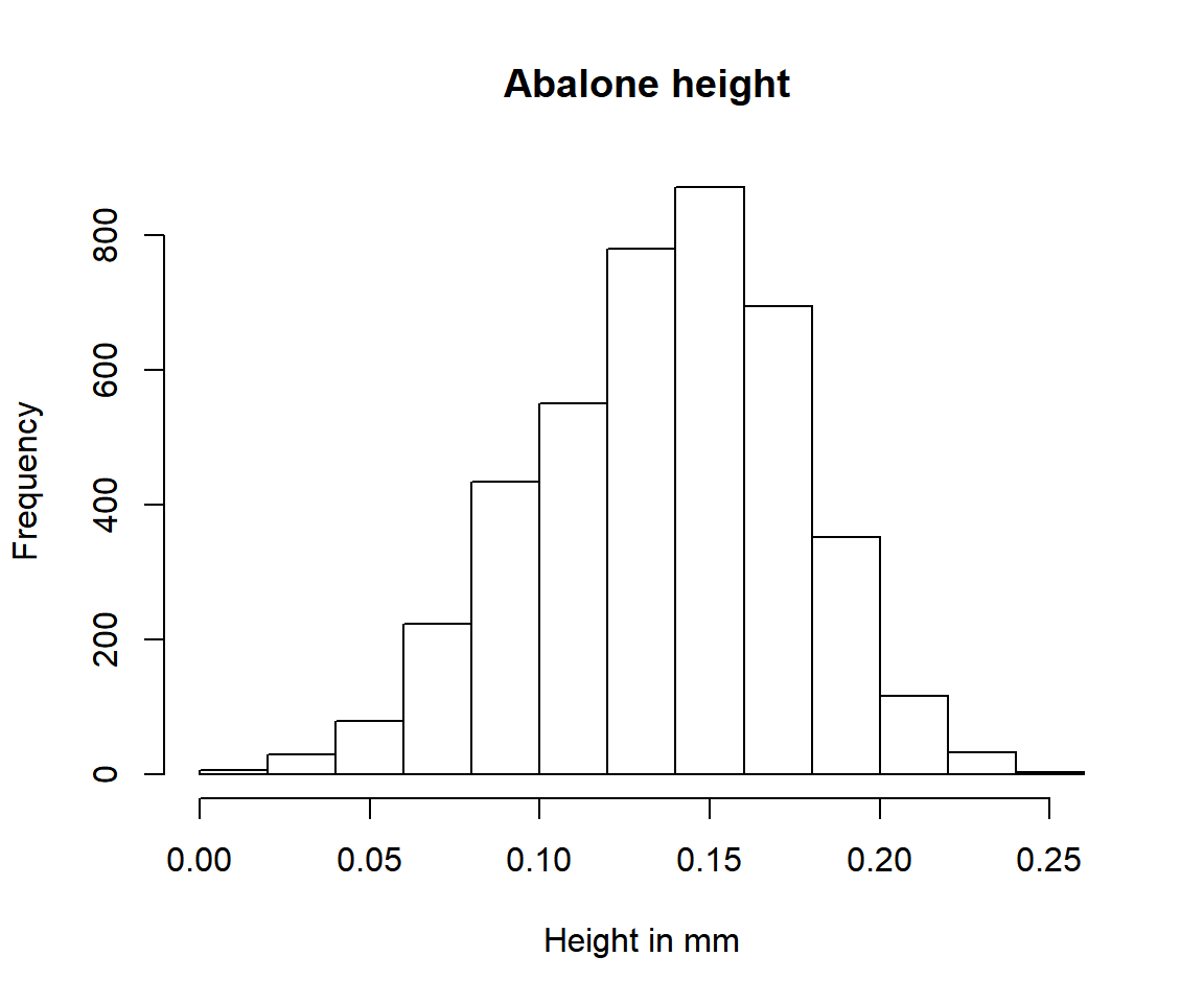
Following Ko, Hjort, and Hobæk Haff (2019) we will take a look at four measurements of the abalones, namely diameter, height, shell_weight and age. The variable age is not present in the abalone data, but is defined as age = rings + 1.5. Moreover, there are two outliers in the height data at at \(1.13\) and \(0.52\). We will remove these outliers.
data = dplyr::filter(abalone, height < 0.5)
data$age = data$rings + 1.5
hist(data$height, main =" Abalone height", xlab = "Height in mm")
Let’s continue doing step 1. First we must decide on a set of models to try out.
models = c("mlgumbel", "mllaplace", "mllogis", "mlnorm", "mlexp", "mlgamma",
             "mlinvgamma", "mlinvgauss", "mlinvweibull", "mlllogis", "mllnorm",
             "mlrayleigh", "mlweibull", "mllgamma", "mlpareto", "mlbeta", "mlkumar",
             "mllogitnorm")
length(models)
## [1] 18The nest step is to define a function that calculates the AIC for all our candidate models over every margin.
#' Calculate AICs for a column
#' @param variable The variable to calculate AICs for.
#' @return A named vector of AICs.

AICs = function(variable) {
  x = data[[variable]]
  FUN = function(name, x = NULL) tryCatch(expr = eval(call(name, x)),
                                                 error = function(e) NULL)
  fits = Filter(Negate(is.null), sapply(X = models, FUN = FUN, x = x))
  sort(sapply(fits, AIC))
}
This function returns a vector of AICs for each model where ml*** didn’t fail. When it fails it is since the support of the data doesn’t not match the density, for instance when -1 is fed to the exponential density.
##      mllnorm     mlgumbel   mlinvgauss     mllgamma      mlgamma
##     21033.17     21039.99     21055.60     21100.20     21104.82
##   mlinvgamma      mllogis    mllaplace       mlnorm    mlweibull
##     21107.62     21295.85     21310.76     21627.91     21893.36
## mlinvweibull   mlrayleigh        mlexp     mlpareto     mlllogis
##     22050.05     23860.54     28697.63     31678.23    394429.50
But we are most interested in the models with smallest AICs.
##     diameter       height shell_weight          age
##    "mlkumar"     "mlnorm"  "mlweibull"    "mllnorm"
Now we use the fitCopula from the package copula on the transformed margins of abalone.
We will examine two elliptical copulas and three Archimedean copulas. The elliptical copulas are the Gaussian copula and the t-copula, while the Archimedean copulas are the Joe copula, the Clayton copula, and the Gumbel copula.
# Transform the marginals to the unit interval.
y = as.matrix(dplyr::transmute(data,
                     diameter = pml(diameter, mlkumar(diameter)),
                     height = pml(height, mlnorm(height)),
                     shell_weight = pml(shell_weight, mlweibull(shell_weight)),
                     age = pml(age, mllnorm(rings))))

# The copulas described above.
copulas = list(normal = copula::normalCopula(dim = 4, dispstr = "un"),
               t = copula::tCopula(dim = 4, dispstr = "un"),
               joe = copula::joeCopula(dim = 4),
               clayton = copula::claytonCopula(dim = 4),
               gumbel = copula::gumbelCopula(dim = 4))

fits = sapply(copulas,
              function(x) copula::fitCopula(x, data = y, method = "mpl"))

sapply(fits, AIC)
## normal t joe clayton gumbel
## -20776.28 -21856.69 -10139.89 -14546.95 -13586.67The t-copula is the clear winner of the AIC competition. The Archimedean copulas perform particularly poorly.
Hence our final model is the t-copula with Kumaraswamy (mlkumar) marginal distribution for diameter, normal marginal distribution for height, Weibull marginal distribution for shell_weight, and log normal marginal distribution for age.