Density, distribution function, quantile function and random generation for a univariate distribution estimated by maximum likelihood.
dml(x, obj, log = FALSE)

pml(q = q, obj, lower.tail = TRUE, log.p = FALSE)

qml(p = p, obj, lower.tail = TRUE, log.p = FALSE)

rml(n = n, obj)
Arguments
| x, q | vector of quantiles. |
|---|---|
| obj | an |
| log, log.p | logical; if |
| lower.tail | logical; if |
| p | vector of probabilities. |
| n | number of observations. If |
Value
dml gives the density, pml gives the distribution
function, qml gives the quantile function, and rml
generates random deviates.
Details
dml is the density, pml is the distribution function,
qml is the quantile function, and rml is the random variable
generator.
These functions work like their counterparts in `stats`, e.g.
Normal. The univariateML object contains both maximum
likelihood estimates and the identity of the model these estimates were
calculated under. These functions are wrappers around underlying density,
distribution, quantile and random generation functions where unknown
parameters are filled with the maximum likelihood estimates.
See the example.
Examples
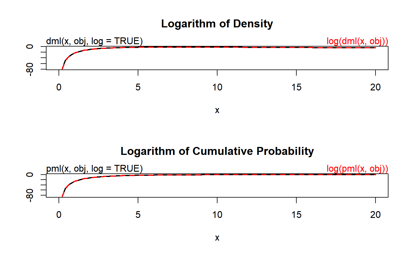
## Simple example obj <- mlnorm(airquality$Wind) dml(0.5, obj) == dnorm(0.5, mean = obj[1], sd = obj[2])#> [1] TRUE## We study the Beta prime model applied to the airquality data set. obj <- mlbetapr(airquality$Wind) ## Example copied from 'stats::dnorm'. par(mfrow = c(2, 1)) plot(function(x) dml(x, obj, log = TRUE), from = 0, to = 20, main = "Logarithm of Density", ylab = NA, lwd = 2 ) curve(log(dml(x, obj)), add = TRUE, col = "red", lwd = 2, lty = 2) mtext("dml(x, obj, log = TRUE)", adj = 0) mtext("log(dml(x, obj))", col = "red", adj = 1) plot(function(x) pml(x, obj, log = TRUE), from = 0, to = 20, main = "Logarithm of Cumulative Probability", ylab = NA, lwd = 2 )